scBench is a suite of 394 rule-scored checks for automated agents working on single-cell RNA sequencing data. Its public canonical slice (thirty tasks across five sequencing platforms and seven task types, scored only by deterministic graders) was ported into inspect_evals.
The port proved harder than expected and more informative than headline accuracy alone. This article focuses on three themes: which engineering choices actually mattered, how small differences in the evaluation setup (the software that runs the model, applies tools, and records scores) shifted outcomes, and what run logs (the stored message history for each task) revealed when failures were read closely.
Table of Contents
- What is scBench, briefly
- Why port it to inspect_evals
- The anatomy of the port
- The grader re-implementation
- Harness differences that mattered more than model choice
- Results on the canonical 30
- Run logs: where failures show up
- The MissionBio trap
- Statistical considerations on small samples
- Lessons for benchmark portability
What is scBench, briefly
scBench (Workman et al., 2026) gives an automated agent a standard single-cell data file (.h5ad) and an instruction in ordinary language, such as filtering low-quality cells or reporting a biological quantity, then compares the agent’s structured answer file to the reference using a fixed scoring program. There is no partial credit by human judgment and no separate “judge” model. The full benchmark contains 394 tasks; the public canonical subset contains thirty.
Tasks are designed so that answers must come from working with the actual dataset: shortcuts such as shipping precomputed embeddings or cached labels are removed, and correct responses depend on quantities specific to each file. An agent that knows library APIs in the abstract but never loads the file will still fail.
The paper evaluates models with mini-SWE-agent, a loop in which the model writes shell-backed code blocks and the evaluation software executes them. The question taken up here is how behavior and scores change when the same tasks are run inside Inspect’s tooling, and whether the thirty-task slice still supports meaningful conclusions.
Why port it to inspect_evals
Three motivations:
Open reproduction. The original pipeline relied on vendor-hosted file locations and fixed hardware. The port targets data hosted on Hugging Face, execution inside a standard container, and no dependence on a single vendor’s infrastructure.
Comparing models fairly. Inspect allows switching the model with one command-line flag. The original stack needed custom wiring for each agent family.
Structured run logs. Inspect records each message, tool call, and token count in a uniform format. Together with Inspect Scout for automated scans over those logs, failure types can be summarized more systematically than by opening raw JSON files by hand.
The anatomy of the port
The inspect_evals addition lives under src/inspect_evals/scbench/ and includes:
dataset.py: Reads the thirty canonical task definitions, normalizes inconsistent labels for task type (for exampledimension_reductionversusdimensionality_reduction), and builds Inspect samples (single evaluation units).data_manifest.py: Maps former Latch file identifiers to files onretroam/scbench-data. A setup step downloads each task’s.h5adinto the container before the agent starts. Some files are very large (about 1.5 GB for Chromium examples), so timeout settings required care.scorer.py: Readseval_answer.jsonfrom the container and calls the matching scorer. The original behavior is preserved: only an on-disk answer file counts. Answers appearing only in chat text do not.graders/: New implementations of five scorer families fromlatch-eval-tools: numeric tolerance, multiple choice, marker-gene precision and recall, label-set overlap, and distribution comparison. Each follows the same numerical tolerances as upstream.Container image: A
Dockerfilebased onpython:3.12-slimwith common scientific Python libraries (Scanpy, AnnData, HDF5 bindings, NumPy, Pandas, SciPy, scikit-learn, graph and embedding tools), plus Node.js anduvso agents can install tools if needed. Limits were set to four CPUs and sixteen GB RAM.Agent routing: The
agentsetting can invoke mini-SWE-agent, Claude Code, or OpenAI Codex throughinspect-swe, which runs the upstream agent inside the container. Ifinspect-sweis absent, a simpler fallback exposes separatebash()andsubmit()steps.
The grader re-implementation
Rebuilding five scorer families was mostly routine until corner cases appeared.
Numeric tolerance. The numeric scorer allows absolute, relative, minimum, and maximum tolerance modes, possibly asymmetric, across several fields. Agents sometimes emit strings such as "6420" instead of numbers, or booleans where an integer is expected. Each conversion rule had to match the reference implementation or scores would disagree line by line.
Gene names. The marker-gene scorer lowercases names before comparison. That single convention decides whether PTPRC matches ptprc. Behavior was checked against upstream tests drawn from the canonical tasks.
Cell-type proportions. Every reported proportion must fall within tolerance. Missing one category fails the whole item, which is strict but avoids rewarding answers that omit rare groups.
Unit tests were added per scorer, alongside a setup parity test (test_harness_parity.py) that compares prompts, tools, and resource settings against the original stack.
Harness differences that mattered more than model choice
The clearest lesson is that small changes in evaluation setup can move scores on the same tasks more than swapping models. The differences below surfaced when thirteen overlapping tasks were run both in the original scBench setup and in inspect_evals.
1. Whether Python state persists between steps
In mini-SWE-agent, code is often submitted as a multi-line shell block:
python3 << 'EOF'
import scanpy as sc
adata = sc.read_h5ad("data.h5ad")
print(adata.shape)
EOF
Each such block starts a new interpreter process, but agents usually place a full script in one block. The first inspect_evals fallback exposed separate bash() and python() calls where each python() call was a fresh process. Variables such as adata vanished between calls, producing NameErrors unrelated to scientific skill. Routing work through bash() alone, or running the real mini-SWE-agent via inspect-swe, removed this artifact.
2. System prompt wording
The original prompt is deliberately neutral: “You are a helpful assistant that can do anything.” The first Inspect prompt named bioinformatics and listed libraries, which tells the model the domain before it reads the task and unfairly helps it. The skew was documented, and prompts were later aligned for fair comparisons.
3. How message limits are counted
The original step_limit=100 ties one step to one assistant reply plus one observation (on the order of two hundred messages total). Inspect’s message_limit=100 counted every message, roughly halving allowable turns. Long analyses suffered first.
4. Whether chat text can substitute for an answer file
The scorer does not parse answers from free text when eval_answer.json is missing; the score is zero, as in the original. A short experiment that rescued answers from <EVAL_ANSWER> tags in chat raised pass rates by about ten percent because sloppy runs still received credit. That path was dropped to stay aligned with the reference behavior.
5. How much tool output is retained
Inspect truncated tool output at sixteen kilobytes by default; the original allowed about one megabyte with long-line clipping. Large printed tables could be cut mid-stream without an explicit error, so the model might continue on incomplete output.
Score agreement on the overlap
Across thirteen tasks scored under both setups (original Haiku versus Inspect Haiku):
- Some tasks matched on pass versus fail.
- Several disagreed for the reasons above.
- Two original runs failed because no answer file was written.
Inspect sometimes scored higher (cleaner isolation between tasks) and sometimes lower (stricter limits or truncation).
Takeaway: a port moves the questions and the conditions under which answers get produced and read.
Results on the canonical 30
All thirty canonical tasks were run through inspect_evals with multiple models. Aggregated thirty-task runs:
| Model | Accuracy | Stderr |
|---|---|---|
| openai/gpt-5.1 | 43.3% | 9.2% |
| google/gemini-3-pro-preview | 36.7% | 8.9% |
| anthropic/claude-sonnet-4-5 | 30.0% | 8.5% |
The same thirty tasks in the original scBench setup with mini-SWE-agent:
| Model | Accuracy (minisweagent) |
|---|---|
| claude-sonnet-4-5 | 50.0% (15/30) |
| gemini-2.5-pro | 36.7% (11/30) |
The figures below summarize those February 2026 mini-SWE-agent runs: pass and fail come from stored batch results; token totals come from one exported conversation log per task. Each model completed thirty tasks.
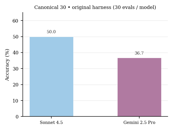
Sonnet’s thirty percent under Inspect versus fifty percent under the original setup reflects evaluation differences above, especially the fallback agent path that split shell and Python across separate tools instead of the bundled mini-SWE-agent loop. After evaluation was routed through inspect-swe with the upstream agent binary, the numbers moved toward parity.
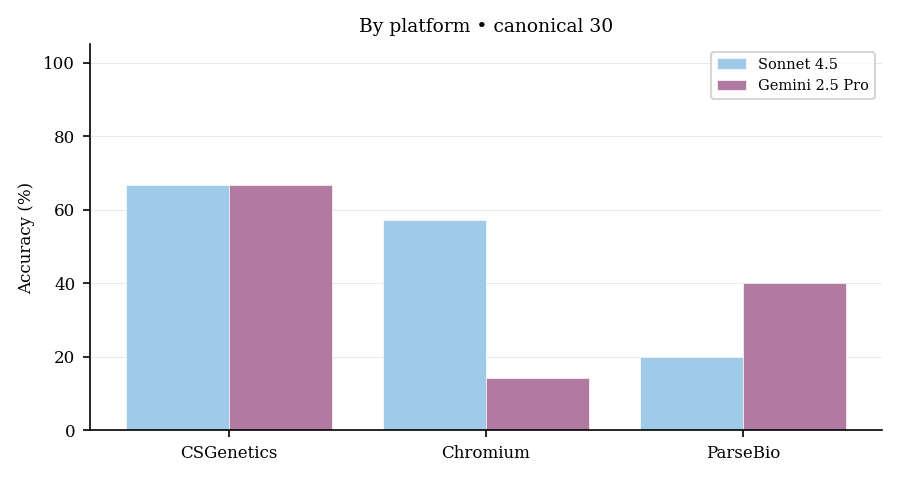
Breakdown by platform
Pooled across inspect_evals runs (181 scored attempts across models and repeats):
| Platform | Accuracy |
|---|---|
| CSGenetics | 60.0% |
| Illumina | 51.6% |
| Chromium | 38.6% |
| ParseBio | 30.8% |
| MissionBio | 25.0% |
The rank order matches the published benchmark (easiest to hardest along this axis): CSGenetics first, MissionBio last. That consistency supports using the thirty-task slice as a coarse health check.
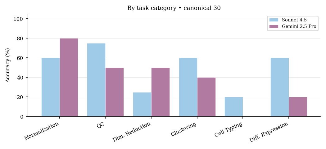
Breakdown by task category
| Task Category | Accuracy |
|---|---|
| Normalization | 53.6% |
| Dimensionality Reduction | 50.0% |
| QC | 47.6% |
| Clustering | 44.4% |
| Differential Expression | 40.0% |
| Trajectory Analysis | 20.0% |
| Cell Typing | 11.5% |
The ordering partly matches the paper (normalization easier than cell typing), but cell typing and trajectory tasks look much harder here than in the full benchmark, likely because the small slice contains few examples per category and a single failure moves the percentage sharply.
Run logs: where failures show up
The most informative material was not aggregate accuracy but reading run logs. Manual review of mini-SWE-agent exports was combined with automated passes over Inspect-format logs.
Failure type taxonomy
Manual labels on all sixty logs (Sonnet 4.5 and Gemini 2.5 Pro, original setup):
| Failure Type | Count |
|---|---|
| Success | 26 |
| Data loading failures | 20 |
| Import errors | 13 |
| Wrong answer | 8 |
| Timeout | 7 |
| NameError | 7 |
| KeyError | 6 |
| File not found | 2 |
| Memory error | 2 |
Data loading failures were the single largest bucket, ahead of logically wrong answers. Models often failed before analysis because they could not open or interpret the file format, not because the biology was too hard.
The verbose-efficient split
Summary statistics:
| Metric | Sonnet 4.5 | Gemini 2.5 Pro |
|---|---|---|
| Pass rate | 50.0% | 36.7% |
| Mean assistant messages | 2.9 ± 2.1 | 6.1 ± 6.1 |
| Mean observations | 2.8 ± 2.0 | 5.9 ± 6.0 |
| Mean total tokens | 30,748 | 125,275 |
| Mean cost per eval | $0.118 | $0.304 |
| Mean duration | 138.7s | 328.4s |
Sonnet passed more often while using fewer turns, tokens, and dollars. Gemini cost about 2.6 times as much per task while passing thirteen points less often.
Token efficiency by outcome
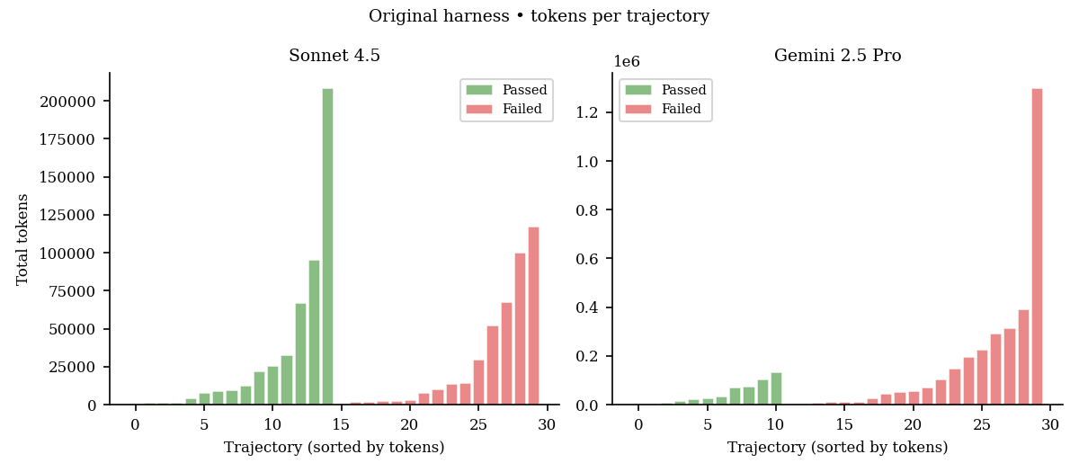
Means by outcome:
| Sonnet (tokens) | Gemini (tokens) | |
|---|---|---|
| Passed | 33,152 ± 55,501 | 44,513 ± 43,787 |
| Failed | 28,345 ± 38,264 | 172,031 ± 298,108 |
Failed Gemini runs used about four times as many tokens as its passes, reflecting long, repetitive retries. Sonnet’s pass and fail totals were closer, consistent with either finishing quickly or stopping early when stuck.
Gemini also split reasoning tokens (internally attributed completion budget): roughly 22,267 on fails versus 11,810 on passes. Higher reasoning volume did not translate into higher pass rates here.
Error recovery patterns
Logs were searched for phrases such as “let me try,” “that failed,” and “alternative approach.”
- Sonnet 4.5: seventeen of thirty logs contained explicit recovery language.
- Gemini 2.5 Pro: ten of thirty.
Sonnet both attempted recovery more often and succeeded more often when it did.
Prompt token growth
Early-turn context size differed:
Sonnet 4.5 (first five assistant turns): prompt size grew from 528 tokens at turn 0 to 19,975 by turn 4.
Gemini 2.5 Pro (same window): 510 tokens to 12,071.
Sonnet tended to emit larger code blocks and receive larger observations each step; Gemini took smaller steps but many more of them, which explains its higher total tokens despite slower growth early on.
Automated scanning with Inspect Scout
Four scanners were run on Inspect logs:
- Answer file: missing or invalid
eval_answer.json. - Environment: import failures, permissions, missing packages.
- Data loading: HDF5 or
.h5adread errors. - Behavior review: a separate strong model flagged confusion or off-topic work.
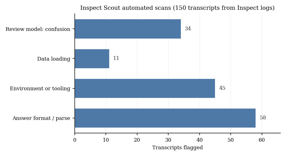
The chart summarizes one archived Inspect Scout run over 150 transcripts taken from Inspect .eval logs for scBench. The height of each bar is how many transcripts triggered that scanner at least once; the same transcript can count toward more than one bar. The first three scanners use pattern matching on log text; the fourth sends the transcript to another model and asks whether the run looked confused or off task.
That fourth step surfaced cases simple pattern rules missed, such as correct loading followed by an irrelevant analysis, or a partial numeric answer never written to the required file.
The MissionBio trap
One instructive failure mode uses MissionBio Tapestri files. They use the .h5ad suffix but are not standard AnnData objects; internally they organize DNA, counts, and protein layers in a nested HDF5 layout.
Most models first call sc.read_h5ad("data.h5ad") and receive:
TypeError: string indices must be integers, not 'tuple'
That message does not state “wrong file type.” Success requires noticing the mismatch, opening the file with h5py, and navigating the assay hierarchy, including separate barcode spaces per sample.
Separate verification confirmed that the file checksum and structure match the intended task asset. The misleading extension reflects how the original hosting labeled downloads; treating it as ordinary AnnData is part of the task design.
MissionBio tasks averaged about twenty-five percent accuracy across models, near half the overall mean. Passing runs pivoted to low-level HDF5 access after reading the traceback; failing runs often repeated read_h5ad with tweaked arguments or exhausted the retry budget without changing strategy.
Statistical considerations on small samples
Thirty tasks raise obvious sampling questions. Following Miller (2024), variance components were estimated for Claude Haiku across five repeats:
- Within-sample variance (run-to-run noise on the same task): 0.0933.
- Between-sample variance (spread of difficulty across tasks): 0.1797.
Resampling suggested six repeat batches as a practical balance for stable accuracy estimates.
The production sweeps used one to three repeats, so uncertainty bands are wider than ideal. Between-task variance nearly doubling within-task variance implies real spread in difficulty, which is desirable even in a small public slice.
Approximate nine-point standard errors separate forty from sixty percent accuracy but not forty from forty-five. Declaring a winner among similar models on thirty tasks alone is unreliable; finer comparisons need the withheld full set of 394 tasks.
Lessons for benchmark portability
1. The evaluation setup defines the benchmark
The thirty JSON task files and scoring code initially looked like “the benchmark.” In practice, the benchmark also includes prompt text, which tools exist, whether interpreter state persists, timeouts, how much output is kept, container contents, and how answers are collected. Changing any layer changes measured skill.
That observation generalizes to any agent benchmark where the model writes executable code in a loop: every loop detail is part of the test specification. scBench documents its choices carefully; this work mainly quantifies how sensitive scores are to those details.
2. Require answer files by default
Pulling answers from chat when the JSON file was missing raised scores about ten percent and rewarded incomplete workflows. If the task demands a file on disk, missing that file should fail, both for realism and for comparable numbers across labs.
3. Small public slices can still track qualitative patterns
Despite only thirty tasks, the slice reproduced broad patterns from the paper (platform ordering, easier normalization than cell typing, stable model ranking at coarse resolution). It is weak for ranking similar models but strong for spotting which failure modes dominate.
That division of labor (small open slice, large private set) is a sensible release pattern.
4. Format diversity stresses models more than sheer size
The hardest platform here is not necessarily the largest file but the one with an unusual on-disk layout (MissionBio). Benchmarks aimed at robust assistants should emphasize several real file organizations rather than one format at extreme scale.
5. Token use tracks outcomes
The model with fewer turns, tokens, and dollars per task also passed more often in these logs, both across models and within each model between passes and failures. Long, rambling runs were usually a sign of trouble rather than careful reasoning.
Code for the Inspect integration: inspect_evals/scbench. Canonical task inputs: retroam/scbench-data. To rebuild the figures, use the notebooks under retroam/scbench/tree/main/notebooks; they reload the stored batch summaries and per-task conversation exports referenced above.
scBench is by Kenny Workman, Zhen Yang, Harihara Muralidharan, Aidan Abdulali, and Hannah Le at LatchBio. The inspect_evals port was contributed by @retroam.